Trading Stocks with Q-Learning
In order to learn more about reinforcement learning, I decided I'd try to train a Q-Learning agent to trade stocks. One of the nice things about using reinforcement learning to trade stocks vs. regression is that the agent makes the decisions for you (as opposed to simply a prediction) about when to take an action and how long to hold a position, which takes the human element out of the loop. For someone like myself with not a lot of professional trading experience, this is perfect. By using reinforcement learning, a policy can be learned which makes decisions that optimizes rewards.
The main approach I took was to compare a trading policy based on a fixed set of rules vs. a trading policy implemented using a trained Q-Learning agent. The fixed rule approach was implemented using a logical condition based on a set of commonly used technical indicators, while the Q-Learning agent would be trained on those same indicators. I'd use the same stock data to train and evaluate both policies and assume that for the sake of simplicity, one 1 stock could be included in my portfolio.
The fixed rule strategy I created beat the benchmark portfolio for both in sample and out of sample periods,although not by much. For both instances, only a few trades were made. The plots below show performance vs. benchmark and the different entry points. Risk adjusted return was similar for the in sample periods, but for the out of sample period, the strategy provided a significant improvement over the benchmark.
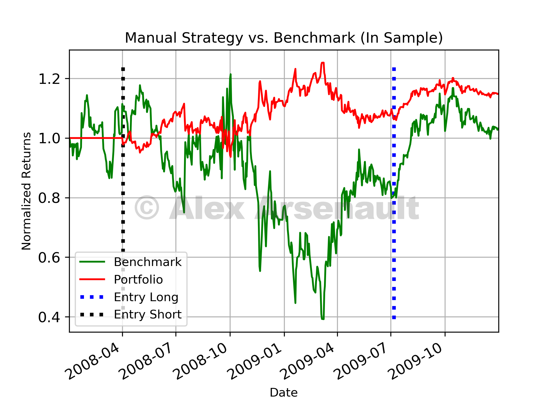 Manual fixed strategy in sample performance.
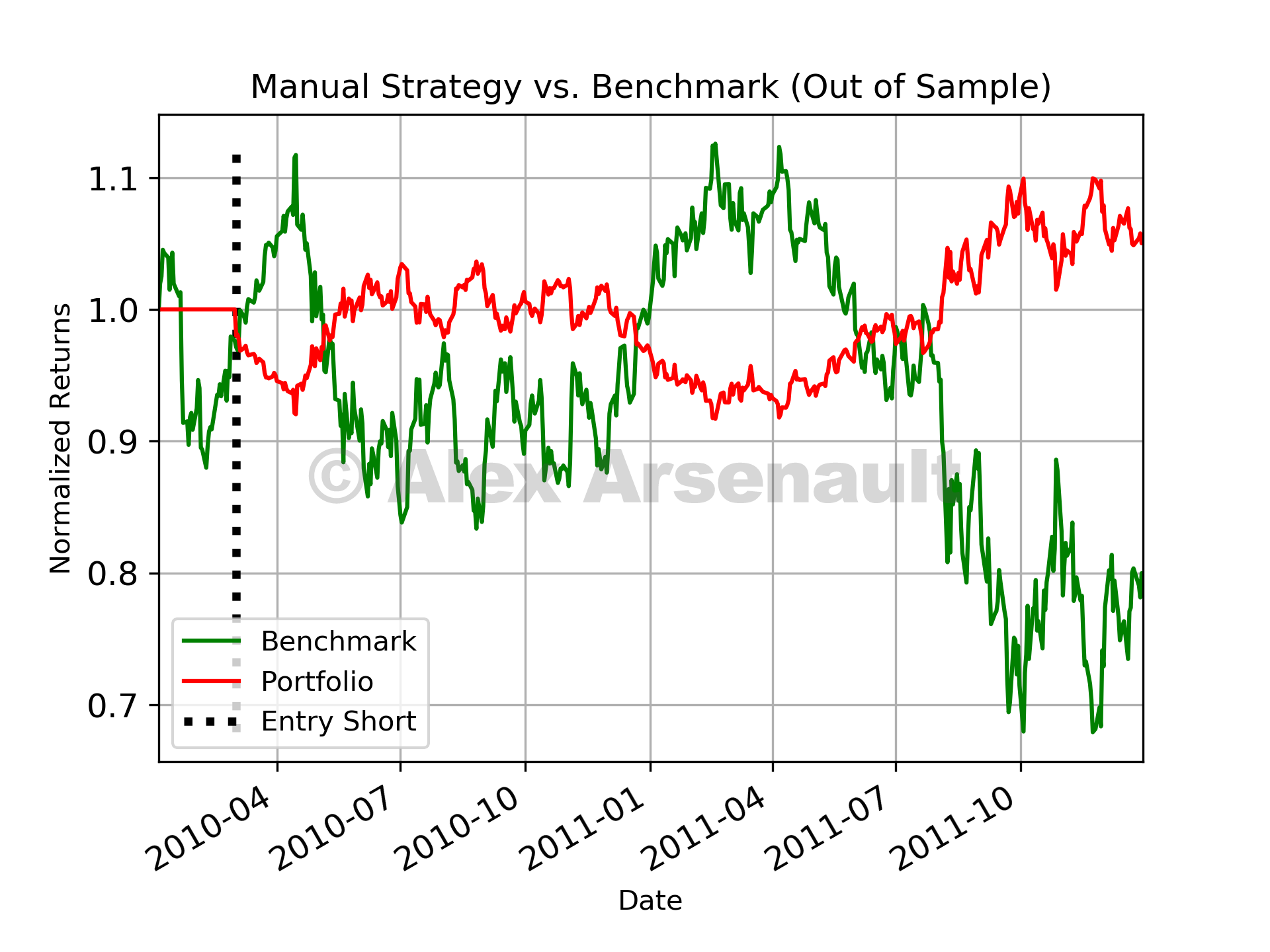 Manual fixed strategy out of sample performance.
In order to use reinforcement learning for trading, the problem needed to be framed as a deterministic Markov Decision Process (MDP). In order to do this, the relevant information was broken down into states, actions, and rewards. Q-Learning aims to update a Q-table (a function of state, and action) through the process of exploration and observation as described below. Once the Q-table is sufficiently trained, it can be used to take actions based on the current state that maximizes future rewards.
- Q-table is initialized to all 0’s
- Current state, s, is observed
- Select some action, a, and execute it
- Observe the immediate reward, r, and the new state, s’
- Q-table is updated according to Eq. 1
- State is updated and steps 2-6 are repeated until total reward converges
Q[s,a] = Q[s,a] + ⍺(r(s,a) + *argmax(Q[s',a])-Q[s,a]) Eq. 1
In this analysis, states were considered to be an abstraction of the technical indicator values, and current portfolio position at that time. In order to quantify these states, the indicator values were each discretized into 10 equal sized buckets using the pandas ‘qcut’ function. Then, for each step in time the combination of bucket numbers associated with each technical indicator and current portfolio position was mapped to a single integer value using a mapping function.
In this market simulation, three possible actions were considered to be possible: take a long position, take a short position, or hold the current position. Rewards were considered to be the daily return of the portfolio as a result of the current position. For example, if a long position is taken and the price of the stock goes up, then the reward is positive and is computed as the value of the shares held multiplied by the percentage increase in stock price. Rewards for short positions are computed similarly, however for short positions decreases in stock price lead to positive rewards. The hyper-parameters used for the Q-Learner and their chosen values were:
- ⍺ (learning rate): 0.2 - Specifies how much new Q-values are weighted vs. old ones during the Q-table update process.
- 𝛾 (discount factor): 0.9 - How much much future rewards are valued vs. immediate rewards during Q-table update process.
- Random action rate (rar): 0.98 - How often are random actions taken during exploration phase.
- Random action decay rate (radr): 0.999 - How quickly do we transition out of the random action (exploration) phase.
- Dyna: 200 - How many dyna iterations are used in an attempt to learn a model of the environment.
Once trained, the Q-Learning approach actually performed pretty well (at least for in sample data). You can see the plot of Q-Learning performance vs. fixed rule strategy vs. benchmark below. For out of sample data, the Q-Learning performance was pretty inconsistent, so you probably shouldn't bet your life savings on this technique! Overall, it was pretty cool to build a Q-Learning agent and see it perform so well for the in sample period. I'm currently working on bolstering this approach using a deep Q-Learning techniques where the transition and reward functions are approximated using neural networks. Maybe with this approach and some added complexity I might be able to see some real performance on out of sample data! Feel free to check out all the code in my repository here.
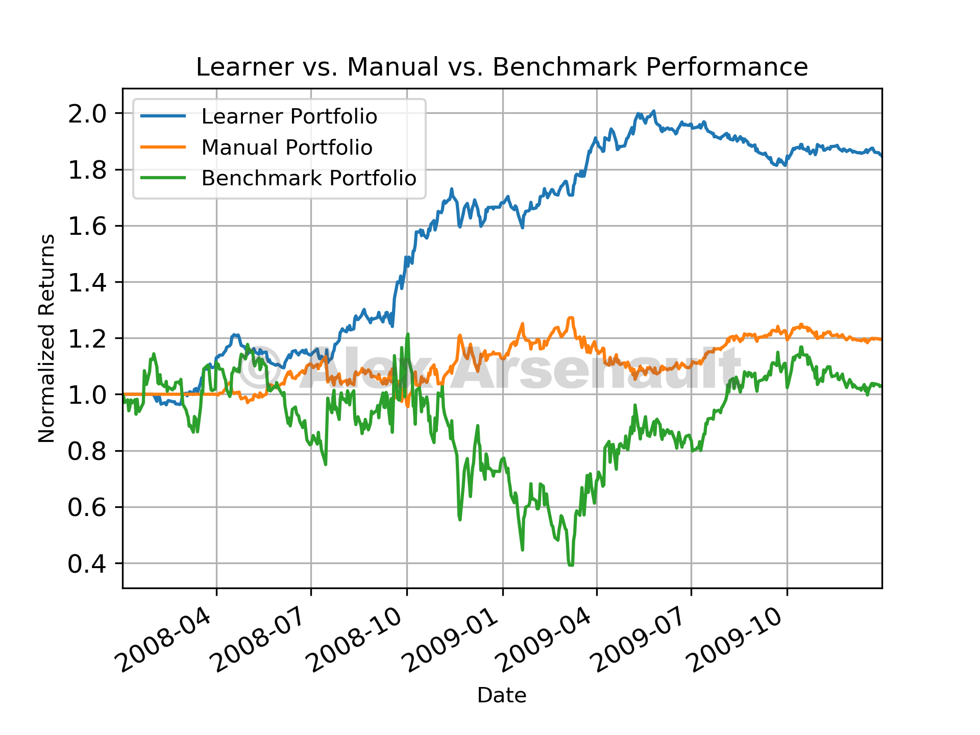 Comparison of fixed strategy vs. Q-Learning vs. benchmark.